Preference elicitation approach for measuring the willingness to pay for liver cancer treatment in Korea
Article information
Abstract
Background/Aims
The Korean government has expanded the coverage of the national insurance scheme for four major diseases: cancers, cardiovascular diseases, cerebrovascular diseases, and rare diseases. This policy may have a detrimental effect on the budget of the national health insurance agency. Like taxes, national insurance premiums are levied on the basis of the income or wealth of the insured.
Methods
Using a preference elicitation method, we attempted to estimate how much people are willing to pay for insurance premiums that would expand their coverage for liver cancer treatment.
Results
We calculated the marginal willingness to pay (MWTP) through the marginal rate of substitution between the two attributes of the insurance premium and the total annual treatment cost by adopting conditional logit and mixed logit models.
Conclusions
The effects of various other terms that could interact with socioeconomic status were also estimated, such as gender, income level, educational attainment, age, employment status, and marital status. The estimated MWTP values of the monthly insurance premium for liver cancer treatment range from 4,130 KRW to 9,090 KRW.
INTRODUCTION
We presumably are unanimous in the belief that cancer disease is one of the most serious and devastating health problems of which the impacts can encompass catastrophic monetary losses as well as premature deaths and many more. According to a statistics report in Korea, the cancer incidence is growing annually by on average 1.8% and the cumulative risk of cancer development during the lifetime is over 37%, which is significantly higher than that of Japan with less than 30%.1
In this regard, the Korean government has been trying to expand the health insurance coverage especially on the treatments of 5 most prevalent cancers (stomach, liver, lung, colon, and breast cancers). And more recently, it enhanced the benefits to 4 major disease categories (cancers, cardiovascular diseases, cerebrovascular diseases, and rare diseases) so that it aims to reduce the financial burden of the cancer patients and their family should incur. On the other hand, however, it is expected that this policy implementation should be a major threat to the insurer's budget in Korea (i.e., NHIS) and eventually lead to a serious financial turmoil in sustaining the policies in medical and health care. Under the universal insurance plan in Korea, the insurance premium is mandated to the insured based on their income or wealth amounts, and the rate of premium hike is determined to reflect the price adjustment of medical care services and coverage enhancement of the fiscal years. So, if the budget expansion is partially or fully transferred to the insured through a premium hike, a substantial resistance from the insured is highly likely.
From the standpoint of the insured, people can recognize the coverage enhancement as cheaper 'out-of-pocket' costs while premium hike as 'extra' monetary burden even though they will realize the former will definitely outweigh the latter once they are diagnosed of corresponding disease(s) that the policy applies.
In our study, the basic question is "how much additional insurance premium are people willing to pay to benefit the coverage enhancement policy?" On this basis, we wanted to investigate the marginal willingness to pay (MWTP) of the people for the increased coverage of cancer treatments. In conducting this research, we adopt 'state-of-the-art' methodology to elicit the preference which is mainly used in estimating the monetary values of 'non-market' goods such as health and environment. In the sense that 'good health' through coverage enhancement is a product which will be chosen probabilistically in the future and additional premium is a price which people are eager to pay to spread the unknown future risks, we are able to elicit the preferences that reflect MWTP. Here, we notify the estimated values of average annual treatment costs of cancers and additional monthly insurance premium so that respondents can reveal their preferences in each given choice set. From this procedure, this study eventually tries to show the reasonable amount of insurance premium for the expansion of cancer treatment coverage. Due to the diversity and differences among the cancer diseases, our study focused only on the liver cancer so that we avoid any spurious or biased estimation results when all types of cancers were included.
DESIGN OF EXPERIMENTS
It is widely understood that there are various treatments available for any specific cancer in most medically developed countries including Korea. These treatments vary with respect to the nature of the procedure and the efficacy, safety profile, outcome, and so forth. Several situations exist where patients face trade-offs between the risks and benefits of alternative treatment methods. To make an informed choice, one needs to be able to weigh up the slight differences in the treatment effectiveness against a spectrum of adverse events associated with alternative treatment strategies and methods. Individuals' preferences for alternative treatments need to be considered in the light of the attributes of the treatments. Conjoint preference elicitation (hereafter PE) method, also known as discrete choice experimentation (DCE), is now being widely used in health care research. It is used in cost-benefit analysis (CBA), assisting policy-makers to assess the 'value for money' of a new health intervention. Importantly enough, valuation can be based upon both health and non-health outcomes. Results may assist with reimbursement decision-making, clinical management, marketing strategies and so forth.
This PE method identifies the key characteristics of alternative treatments, and selects a series of levels for each. In a survey, respondents choose from several options, each of which describes a series of attributes at different levels or values. Expressed based on each respondent's preference, the relative importance and trade-offs among attributes can be assessed through various levels of the attributes. This study used choice experiment with respondents randomly selected from a general population to elicit preferences related to the liver cancer treatments.
Conjoint preference elicitation method
As mentioned previously, the application of PE has been popular in health care, policy feasibility analyses, marketing and economic studies over the past several decades despite some practical issues. Owing to rapid improvement in the computer sciences and software packages, researchers could conduct more rigorous estimation works using sophisticated methods than before. In PE, researchers are required to construct a subset of optimal size of all possible combinations of attribute levels so as to avoid or minimize 'irrational responses', 'protest responses' or 'no-answer responses', all of which are due to fatigue and ignorance of respondents with many survey questions. In fact, our survey instrument involves three attributes with three levels and one attribute with four levels, which or levels that gives a total of 108 (=33×41) possible combinations. If a respondent is asked to choose one of the two possible profiles or options, total 5,778 (=108C2) situations will be possible. In here, we need to design a survey instrument by minimizing the number of choice sets so that respondents feel comfortable to answer without having physical and emotional fatigues and at the same time, this instrument needs to successfully reflect the preferences if 5,778 situations were to be taken from each respondent. In this regard, the orthogonal main effects plan (OMEP) in PE method is most frequently adopted as an optimal solution. The objective of experimental design is to reduce the size of possible choice sets to a manageable number of choice sets for the respondents. Huber and Zwerina2 suggest the 3 properties of OMEP; level balance (equal frequency), orthogonality (independency of the levels of each attribute) and minimal overlap (the probability that an attribute level appears itself in each choice set should be as small as possible). The most common OMEP approach is to use statistical packages such as SPSS or LIMDEP, and this study uses SPSS (it is called 'Orthoplan') to generate an optimal size of choice sets that satisfy three properties of experimental designs. The values in each column indicate the level of corresponding attribute. For each attribute variable, the lowest level is shown as 0 and next level is 1, 2, and 3. Besides, in order to comprise the pairs of choice, we made another option by adding the number generator as explained.
Attributes and levels
We chose four attributes such as 'liver cancer rate (incidence rate of liver cancer)', 'survival rate' (or probability) in 5 years after liver cancer treatment, 'total annual treatment costs' and 'monthly insurance premium'. Also we put 3 levels for the first three attributes and 4 levels for the last attribute in the interest of our study. In selecting the levels of 'liver cancer rate' attribute, we referred to Annual Report of Cancer Statistics (National Cancer Center, 2013)1, Cancer Registration Statistics in Korea (National Cancer Center, 2013)3. In here, the given cancer rates imply the 'annual incidence rate' (new liver cancer cases/100,000 persons). For survival rate, we adopted the values from Cancer Registration Statistics (National Cancer Center, 2013), Berrino et al. (2007)4, and NCI SEER (Surveillance, Epidemiology, and End Result Study) Report (2010)5. In estimating 'total annual treatment costs' levels, we calculated the weighted average value based upon respective treatment protocol and costs of liver cancers listed in liver cancer registration statistics and the number of patients in the group (see Table 1). Here, we showed the total annual treatment costs which included all 'out-of-pocket' payments, the patients' copayment and reimbursement from NHIS by assuming that the coinsurance rate for all uncovered parts would be around 36% (National Cancer Center Report, 2013).

Estimated total annual treatment costs for liver cancer patients
Finally, the estimation of monthly insurance premium was conducted as follows. There were 37,072 new liver cancer cases in year of 2011 responsible for about 2,224 billion KRW of annual treatment costs. After dividing by the numbers of health insurance beneficiaries including premium payers (about 47.5 million people), we get 46,917 KRW of extra burden that each beneficiary needs to share. Based upon the maximum and minimum annual total treatment costs from the National Cancer Center Report, we calculated upper and lower bounds of monthly insurance premium levels using the same method. So the levels of 'monthly premium' attribute are 3,300, 3,700, 4,100, and 4,500 (all in KRW). In addition to four attributes for PE experiments, the study included the questions to capture the socioeconomic status (SES) and antecedent variables of respondents (Survey questionnaire is provided in Supplement 1 for perusal). Based upon these, we are able to stratify and compare the estimation results into several subgroups by gender, income level, education level, location of residence, occupation, and premium payer or dependents of insured (The attributes and their respective levels in this study are described in Supplement 2).
With the completed survey questionnaire, we conducted PE survey with 600 respondents randomly selected from the panel of a private research company in Korea of over 435,000 general populations.
ESTIMATION STRATEGY (ECONOMETRIC METHODS)
During the late 1960s and 1970s, social scientists suggested that we could infer, or 'capture' decision makers' policies and values by observing their decisions over enough circumstances. At that time, psychologists working on a variety of seemingly unrelated problems developed a paradigm by which decision makers' policies might be inferred (Luce, 1959; Luce and Tukey, 1964; Krantz, 1964; Tversky, 1967; Anderson, 1981; Hoffman, Slovic, and Rorer, 1968).67891011 PE approach mainly adopts the logistic model originally proposed by Luce (1959).6 In an economic science, random utility theory (RUT) is a point of departure where PE methodology is employed (McFadden, 1974).12 Individuals make their own choices in order to maximize their utilities given several commodities reflecting different levels of attributes. According to RUT, utilities are considered as random variables composed of deterministic component and random error term (i.e. unobservable individual characteristics and uncontrolled environmental factors).
Given several alternatives of choices, each individual chooses the selection that leads to the highest level of his/her own utility. A simple consumer choice model based on RUT is described as follows
Given that error terms are unknown, the probability of individual's choice of alternative j can be shown as below
For the empirical purpose, we assume that the deterministic component part of indirect utility function is an additive linear function of several types of attributes and observed characteristics written as Vij=β'X. Note that a vector of X is defined over attributes and observable characteristics and β will be empirically estimated.
Conditional logit model
Given the distribution of individual error terms, several types of PE method can be employed depending on the form of the choice model. Among many possible ways, the most widely used PE model is McFadden's conditional logit (CL) model.13 In this model, we impose individual error terms as Weibull distributions, which are independent and identically distributed (IID). So the value (εik-εij) will constitute the logistic probability distribution. And the probability that an individual i makes choice of j among k alternatives (see equation (3)) can be derived using a closed form of cross-sectional conditional logit equation below

Based on the estimated coefficients from CL, the MWTP can be calculated by computing the marginal rate of substitution (MRS) between attribute of interest and the cost factor (i.e. taking the total derivative of the utility index). This "value ratio" is also identifiable between non monetary elements of utility.16
The CL model, however, has several econometric issues and problems. Firstly, it has a tendency of modeling bias due to the assumption of preference homogeneity among individual respondents, in which we don't allow heterogeneity of preferences especially for non market goods. If this is the case, the important information from a variety of choice behaviors and preference heterogeneity can simply be ignored so that the estimation might be inconsistent and biased.1718 The preference heterogeneity can be explained in part by observable and systematic characteristics of the respondents while in part by unobservable components. The former heterogeneity can be captured by CL models while the latter needs to be identified by more general models.19 Secondly, CL assumes the error terms to be independent, also known as 'independent of irrelevant alternatives (IIA).' Thirdly, CL captures the panel data that consists of the choice decisions of each question from the same respondent by assuming IIA, which is identical to the choice decisions of each question from all different respondents.
Mixed logit model
In mixed logit (ML) model, we allow that individuals can have different preferences and finally make different choice decision depending upon the circumstances they face. The utility that an individual i gets from a single choice decision of j can be defined as follows.
The equation (5) is identical to equation (1) of CL unless two major issues exist. First, we use subscript i which indicates the heterogeneity of preferences across individuals while CL does not. Second, along with the original error term of εij, a new error term of μi'zij is added, which captures the characteristics of an individual. So equation (5) is defined as ML model with error-components.20 zij is an observable random vector and μi follows N (0, σi2) and varies with individual preferences. The major issue in equation (5) is that the new error term of μi'zij + εij reflects the dependence of alternatives and heterogeneity across individuals. It means that μi explains individual heterogeneity despite the inclusion of εij that assumes IIA in CL model.
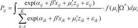
Unlike CL that deals with fixed effects, cross-sectional ML technically cannot get likelihood function. With given variance-covariance matrix Ω*(μi), by integrating the CL probability for all μi values derived from probability density function of f (μi|Ω*), we can get the probability in equation (6)
By adopting two different Logit models above explained, we would like to estimate and compare the MWTP's of insurance premium for the liver cancer treatment.
RESULTS
The PE survey asks the respondents to choose one or more discrete choice options so that we can construct multiple observations for each individual respondent. Since sample size depends on the number of survey participants, the number of choice sets and the number of alternatives in each choice set, the data set from the PE survey should be estimated through various panel data analyses such as fixed effect (FE) models. For each pair-wise comparison of choice set (each respondent will take 16 choice sets), the respondent is asked to make a choice among three alternatives (options A, B, or opt out). Since we treat each choice set faced by each individual and three alternatives as separate outcomes, there are 48 possible outcomes for each individual. So the number of total samples in estimation will theoretically be 28,800 (=600×48) unless we have 'protest bids (i.e., status quo)', 'irrational responses' or 'no answer response' due to various reasons such as anchoring effect or fatigue during the survey, all of which should be dropped out of the sample.
Table 2 shows the summary statistics of the whole samples from the PE survey. The average age of respondents is about 39 ranged from 19 to 59 years old. Male and female respondents are almost equally distributed in the sample. Measured by the formal years of schooling, the educational attainment of respondents shows 14 years in the average level indicating a bit higher than other national statistics in Korea. About 70% of individuals have jobs in the survey period and the proportions of married people are about 66%. The respondents are asked to indicate their salary or income among the 8 categorized interval levels. The average monthly income level of respondents is calculated by taking mid-point value for each category interval, resulting in around 1.82 million KRW.

Descriptive statistics
Table 3 shows the main results from the CL with fixed effects and ML models by controlling only for four attributes such as liver cancer rate, survival rate in 5 years after treatment, total annual treatment costs, and the monthly insurance premium. All of the estimated coefficients except the cancer rate are statistically significant and the joint null hypothesis of all coefficients are being zero is rejected as well based on the log likelihood chi-squared statistic. The direction of coefficients is consistent as the utility theory predicts except the total annual treatment cost variable and liver cancer rate. For example, positive and significant coefficient of survival rate in 5 years after treatment indicates that respondents prefer higher survival rate to lower one after cancer treatment was completed. The respondents obviously prefer smaller extra premium burden for expanded coverage of hypothetical cancer treatment.

Results for the basic conditional logit and mixed logit models
The positive sign of total annual treatment costs does not seem to support for the theoretical validity of the model. However, we put two explanatory variables (total annual treatment costs and monthly insurance premium) related to the measures of cost from cancer treatment in our basic empirical model. Thus, it is not much surprising that we observe the opposite signs between total treatment costs and monthly insurance premium. Given that the coefficients of total treatment costs and monthly insurance premium are opposite directions, we are able to calculate the positive MWTP between those two variables, which is sensible.
And we examine the nature of unobserved heterogeneity (i.e. distribution of error terms in the utility function). The key assumption of CL is IIA which comes from the IID assumption of constant variance. It is obvious that the systematic unobserved components are likely to differ across respondents and as a result they affect the individuals' choice behaviors. There are many ways to relax the IIA assumption. In the paper, we simply try to cure unobserved heterogeneity of each individual by clustering each individual's residuals in the estimation. Table 3 shows the standard error after clustering by each individual in CL model. The authors found out that even though the value of standard error is slightly higher than the unadjusted one, the t-statistic is not significantly different.
Since values of pseudo-R squared of the two logit models are almost the same and bigger than the generally accepted threshold of 0.1, we confirm the two models have both meaningful results.21
Here we try to estimate the MWTP across the several attributes based upon the regression results shown in Table 3. The MRS values are calculated by the negative ratio of any two coefficients. To calculate how much the respondents are willing to pay extra insurance premium on a monthly basis for the full coverage of treatment of all cancers in order to obtain additional 5-year survival opportunity, we should look at the negative ratio of coefficients of survival rate and monthly insurance premium (the denominator part). Therefore, the MWTP for obtaining one additional survival rate in terms of percentage point will be 270.3 KRW which is derived from a calculation of -0.0811/(-0.0003). Therefore, we can interpret that the average respondents are willing to pay extra insurance premium of 2,703 KRW on a monthly basis in return for 10 percentage points increase in 5-year survival rate.
Now our interest also lies in the MWTP between total annual treatment costs and monthly insurance premium. The MWTP between these two variables shows 3,333 KRW which is calculated from a calculation of -0.0001/(-0.0003). Since total treatment cost is measured in ten thousand KRW, the original ratio of 0.333 in ten thousand KRW is rescaled into 3,333 KRW. This shows that the average respondents are willing to pay extra 3,333 KRW of monthly insurance premium for a full coverage of one-year 'direct medical cost' associated with the liver cancer treatment.
As discussed above, the preference heterogeneity needs to be incorporated into the regression models. To resolve the issue, we use 'hybrid' CL model along with mixed logit. To conduct hybrid CL, the SES variables cannot be incorporated as individual explanatory variables in the model because of no variation of them is defined within group each choice set. As an alternative, therefore, we incorporate the interaction term between observed individuals' characteristics and four attributes of our interest. With the insertion of interaction terms, we are allowed to estimate coefficients of each attribute that varies across several sub-categories. Since our main objective is to estimate MWTP of monthly insurance premium, we consider the interaction term for the monthly insurance premium variable. The regression results are presented in the Table 4.

Results for the hybrid conditional logit model with fixed effects
The interaction term is added to the basic model one after another and the results are shown in separate columns. Model 1 includes interaction term between 'female dummy' and 'monthly insurance premium' in order to capture the difference of attitudes on valuing survival rate from liver cancer treatment by gender. The estimated coefficients of three attributes do not change compared to the basic model with only four attributes variables. Interestingly, the size of insurance premium is shown to be quite different between male and female indicating relatively lower WTP in female group than male counterpart.
Before we go any further, we need to check the regression results of ML with the same interaction terms in Table 4 of CL model. We see that the results are almost identical except for being statistically significant with the liver cancer incidence rate. Besides, pseudo R-squared is higher than that of CL model shown in Table 4 and most of them exceed 0.2, which means that ML model is a more appropriate model than hybrid CL with FE.
We now base MWTP estimation on the results shown in Table 5 which uses ML model. The MWTP between survival rate and monthly insurance premium of male is 293.0 KRW (= -0.09084/(-0.00031)), while the MWTP value of the female group is 197.5 KRW (= -0.09084/{(-0.00031) + (-0.00015)}), 32.59% lower than male group. Similarly, the MWTP between total treatment costs and monthly insurance premium can be calculated separately by gender groups. For male, the MWTP is calculated as 6,774 KRW from a calculation of (= -0.00021/(-0.00031)), while the female group has 4,565.2 KRW from a calculation of (= -0.00021/{(-0.00031) + (-0.00015)}) indicating lower by 32.6% than male's one.

Results for the mixed logit model with interaction terms
Model 2 includes the interaction between higher income dummy variable and monthly insurance premium in order to examine the effect of income on the MWTP value. Here, income is defined as high if the respondent's monthly income is more than 4 million KRW which is shown to be at the top 18% level among the whole income range. The coefficient of interaction term appears to be significantly different from low income group. For the low and middle-income groups, the MWTP between survival rate and monthly insurance premium is calculated as 302.2 KRW (= -0.09067/(-0.00030)) and the MWTP for total treatment costs is estimated as 6,333 KRW (= -0.00019/(-0.00030)). Compared to this amount, both the MWTP for survival rate and the MWTP for total treatment costs are lower in high income groups with 197.1 KRW (= -0.09067/{(-0.00030) + (-0.00016)}) and 4,130.4 KRW, respectively. This result seemingly contradicts to our conjecture based on the traditional economic theory, but it is understood that higher income group with more advantageous benefits provided by the private insurance plans are less likely to show more MWTP than its counterparts.
The result with the interaction term of education dummy is presented in the Model 3, of which the estimated coefficient however is not shown to be statistically significant. The results suggest that the educational attainment is not a significant factor affecting the respondents' choice behavior. As results, the MWTP between attributes considered do not substantially change. The MWTP between survival rate and monthly insurance premium is calculated as 246.1 KRW (= -0.09104/(-0.00037)) and the MWTP for total treatment costs is estimated as 5,405.4 KRW (= -0.00020/(-0.00037)).
Model 4 includes the interaction term of age dummy (50 and older), of which the coefficient is statistically insignificant. The MWTP between survival rate and monthly insurance premium is calculated as 259.7 KRW (= -0.09090/(-0.00035) ) and the MWTP for total treatment costs is estimated as 6,000 KRW (= -0.00021/(-0.00035)).
Model 5 includes the interaction term of employment status dummy. For the samples having no jobs, the MWTP for survival rate is calculated as 190.0 KRW (= -0.09121/(-0.00048)) and the MWTP for total treatment costs is estimated as 4,166.7 KRW (= -0.00020/(-0.00048)). Compared to this amount, both the MWTP for survival rate and the MWTP for total treatment costs are higher in the group who are currently employed with 414.6 KRW and 9,090.9 KRW, respectively.
Model 6 includes the interaction term of marital status dummy, which shows no significant effect. The MWTP between survival rate and monthly insurance premium is calculated as 266.1 KRW (= -0.09046/(-0.00034)) and the MWTP for total treatment costs is estimated as 5,882.3 KRW (= -0.00020/(-0.00034)).
DISCUSSION & CONCLUSION
By adopting CL and ML models in analyzing the conjoint PE approach, this study aims to measure the MWTP of monthly insurance premium in return of coverage expansion. The simple CL and ML models estimate the MWTP of monthly insurance premium for an expanded coverage of liver cancer treatment cost with respectively 2,000 KRW (from ML) and 3,333 KRW (from CL). And after inserting various interaction terms, we find the MWTP will vary mostly from 4,130 KRW to 9,090 KRW depending on the categories of interaction term. In this vein, this study can contribute to creating a new type of research in helping implement government health care policies. Despite the main objective of the study, we automatically consider the effect of several individual and SES variables such as gender, income level, educational attainment, age, employment status, and marital status on the size of MWTP of insurance premium for reducing total annual treatment costs associated with liver cancer. Among them, gender, income level, and employment status tend to affect the MWTP variation across corresponding groups.
The analysis in this paper provides answers, albeit based on a single data set composed of ordinary people who have never personally been diagnosed of liver cancer, to several questions of the interest to those who want to know how to manage and finance national health insurance budgeting. More precisely, this study tries to figure out how much people are eager to pay if they realize that the beneficial insurance plan can help them avoid a catastrophic financial disaster associated with cancer disease. To sustain the national health insurance plan, insurance premium is inarguably a crucial source and its amount and adjustment should be determined on the evidence basis that sufficiently reflects the willingness to pay as well as affordability of the premium payers.
To the best knowledge of ours, only two researches conducted on this matter. Lee et al.22 firstly tried to simulate and estimate the expected additional burden of insurance premium at both individual and familial levels with given hypothetical conditions of numeric premium rate changes and the hikes in government subsidies with 20%, 30%, or 40% in financing the national health insurance systems. They present that, depending on their insurance types, each individual should incur ranging 12,519 to 23,429 KRW for a coverage expansion of all diseases. Using DCE method with nested logit model, Jo23 firstly conducted the MWTP estimation study to figure out the characteristics of the decision-making for the treatments of all cancer types and investigates the attributes affecting the respondents' choice. He ascertains MWTP and relative preferences for all cancer treatments among the general population. Taking various factors, the study reflects the MWTP ranging from 8,484 KRW to 14,970 KRW.
Like the previous researches on this matter, this study also has some problems and limitations that cannot be overcome. Firstly, in most industrial sectors including health care, there has been ever growing technology dynamics, which our study cannot reflect by simply assuming it to be fixed. Due to bigger dependency on medical technologies, technological progress can lead to higher health costs even though it also results in a longer life with better health. But relatively bigger dependency in medicine tends to make people be price-unconscious and choose higher level of medical technology as long as it is substantially covered. Secondly, the PE method does not account for uncertainty in the calculation of the welfare valuations and the estimates from CL and ML models surely represent the certainty equivalents. When we add uncertainty in estimation procedure, the values will be lower than shown in this study.
Acknowledgements
This study was financially supported by Pfizer Korea, Inc. The authors have no conflicts to disclose. And the publication of study results is not contingent on the sponsor's approval.
Notes
Conflicts of Interest: The authors have no conflicts to disclose.
Abbreviations
CBA
cost-benefit analysis
CL
conditional logit
DCE
discrete choice experimentation
FE
fixed effects
IIA
independent of irrelevant alternatives
IID
independent and identically distributed
ML
mixed logit
MRS
marginal rate of substitution
MWTP
marginal willingness to pay
NHIS
National health insurance service
OMEP
orthogonal main effects plan
PE
preference elicitation
RUT
random utility theory
SES
socioeconomic status
References
SUPPLEMENTARY MATERIALS
Supplementary data related to this article is available online http://e-cmh.org/suppl/chm-21-3-268-s001.pdf.
Supplementary 1
Survey questionnaire
Supplementary 2
Preference elicitation survey instrument (Excerpt)